
Ordinary Differential Equations (ODEs) in MATLAB
MATLAB provides powerful tools for solving ordinary differential equations (ODEs). ODEs are equations involving derivatives of an unknown function with respect to a single variable. MATLAB offers several functions to solve ODEs numerically, including ode45, ode23, ode15s, and others.
Introduction to ODEs
Consider the general form of an ODE:
dy/dx = f(x, y)
The goal is to find the function y(x) that satisfies this equation, given some initial conditions.
Types of ODEs
MATLAB can handle various types of ODEs, such as:
- First-order ODEs
- Higher-order ODEs
- Systems of ODEs
- Stiff ODEs
Using MATLAB for Solving ODEs
The basic syntax for solving an ODE in MATLAB is:
% Syntax for solving ODEs

[t, y] = solver(@odefun, tspan, y0);
solver: The MATLAB ODE solver (e.g.,ode45,ode23)@odefun: Handle to the function defining the ODEtspan: Vector specifying the time rangey0: Initial condition(s)
Example 1: Solving a First-Order ODE
Consider the ODE:
dy/dt = -2y, y(0) = 1
To solve this ODE in MATLAB:
% Define the ODE function

odefun = @(t, y) -2 * y;

tspan = [0 5];  % Time range

y0 = 1;         % Initial condition


% Solve using ode45

[t, y] = ode45(odefun, tspan, y0);


% Display results

disp([t, y]);


% Plot the solution

plot(t, y);

xlabel('Time t');

ylabel('Solution y');

title('Solution of dy/dt = -2y');
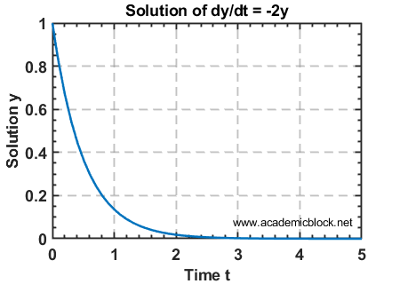
The output would look like:
    t       y
    0.0     1.0000
    0.1     0.8187
    0.2     0.6703
    ...
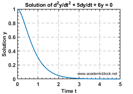
Example 2: Solving a Second-Order ODE
Consider the second-order ODE:
d2y/dt2 + 5dy/dt + 6y = 0, y(0) = 1, dy/dt(0) = 0
This can be rewritten as a system of first-order ODEs:
dy1/dt = y2, dy2/dt = -5y2 - 6y1
% Define the ODE system

odefun = @(t, y) [y(2); -5 * y(2) - 6 * y(1)];

tspan = [0 5];  % Time range

y0 = [1; 0];    % Initial conditions


% Solve using ode45

[t, y] = ode45(odefun, tspan, y0);


% Plot the solution

plot(t, y(:, 1));

xlabel('Time t');

ylabel('Solution y');

title('Second-Order ODE Solution');
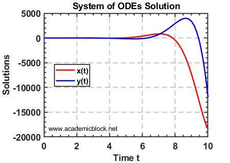
Example 3: Solving Systems of ODEs
Consider the system:
dx/dt = x - y, dy/dt = x + y
% Define the ODE system

odefun = @(t, y) [y(1) - y(2); y(1) + y(2)];

tspan = [0 10];

y0 = [1; 0];


% Solve the system

[t, y] = ode45(odefun, tspan, y0);


% Plot both solutions

plot(t, y(:, 1), '-r', t, y(:, 2), '-b');

legend('x(t)', 'y(t)');

xlabel('Time t');

ylabel('Solutions');

title('System of ODEs Solution');
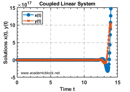
Example 4: Coupled Linear Systems of ODEs in MATLAB
Coupled linear systems of ODEs involve multiple equations that are interdependent. MATLAB provides tools to solve these efficiently using numerical solvers like ode45.
Consider the coupled system:
\[ \frac{dx}{dt} = 3x + 4y, \quad \frac{dy}{dt} = -4x + 3y, \quad x(0) = 1, \quad y(0) = 0 \]
We aim to solve this system for \( t \) in the range [0, 10].
MATLAB Code
% Solve the system using ode45

tspan = [0 10];             % Time range

y0 = [1; 0];                % Initial conditions: x(0) = 1, y(0) = 0

[t, y] = ode45(@coupledODE, tspan, y0);


% Extract and plot the results

plot(t, y(:, 1), '-o', t, y(:, 2), '-x');

xlabel('Time t');

ylabel('Solutions x(t), y(t)');

legend('x(t)', 'y(t)');

title('Solution of Coupled Linear System');

grid on;


% Define the coupled system as a function

function dydt = coupledODE(t, y)

    dydt = [3*y(1) + 4*y(2);  % dx/dt

            -4*y(1) + 3*y(2)]; % dy/dt

end
Explanation of the Code
Step 1: Define the system of equations in the function coupledODE.
Step 2: Specify the time range and initial conditions.
Step 3: Use ode45, MATLAB’s solver for non-stiff ODEs, to compute the solution.
Step 4: Extract and plot the solutions for visualization.
Expected Output
Running the code will generate a plot showing the evolution of \( x(t) \) and \( y(t) \) over time.
Plot
The plot will illustrate the coupled nature of the solutions, where changes in one variable affect the other.
Example 5: Using Laplace Transforms to Solve ODEs in MATLAB
The Laplace Transform method is a powerful analytical tool for solving linear ordinary differential equations. MATLAB’s Symbolic Math Toolbox simplifies this process significantly.
Consider the second-order ODE:
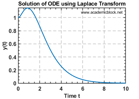
\[ y” + 3y’ + 2y = 4e^{-t}, \quad y(0) = 1, \quad y'(0) = 0 \]
We will solve this ODE using the Laplace Transform.
MATLAB Code
% Define the symbolic variables

syms y(t) Y s


% Define the ODE

ODE = diff(y, t, 2) + 3*diff(y, t) + 2*y == 4*exp(-t);


% Apply Laplace Transform to the ODE

ODE_Laplace = laplace(ODE, t, s);


% Substitute initial conditions: y(0) = 1, y'(0) = 0

ODE_Laplace = subs(ODE_Laplace, [laplace(y(t), t, s), y(0), subs(diff(y(t), t), t, 0)], [Y, 1, 0]);


% Solve for Y(s) in the Laplace domain

Y = solve(ODE_Laplace, Y);


% Apply Inverse Laplace Transform to find y(t)

y_sol = ilaplace(Y, s, t);


% Display the solution

disp('Solution of the ODE:');

disp(y_sol);


% Plot the solution

fplot(y_sol, [0, 10]);

xlabel('Time t');

ylabel('y(t)');

title('Solution of ODE using Laplace Transform');

grid on;
Explanation of the Code
Step 1: Define the symbolic variables and the ODE.
Step 2: Apply the Laplace Transform to the ODE using MATLAB’s laplace function.
Step 3: Substitute the initial conditions into the Laplace-domain equation.
Step 4: Solve for \( Y(s) \) and apply the inverse Laplace Transform using ilaplace to find \( y(t) \).
Step 5: Visualize the solution with fplot.
Expected Output
The solution for \( y(t) \) will be displayed as a symbolic expression, and a plot of \( y(t) \) over the interval \( [0, 10] \) will be generated.
    Solution of the ODE:

    (2*exp(-t))/3 + exp(-2*t) - (2*exp(-t)*t)/3
Plot
The plot will illustrate the behavior of \( y(t) \), showing how the solution evolves over time.
Initial Value Problems (IVPs) in MATLAB
MATLAB provides powerful tools to solve Initial Value Problems (IVPs) numerically. This example demonstrates solving a first-order ODE using the ode45 solver.
Example Problem
Consider the IVP:
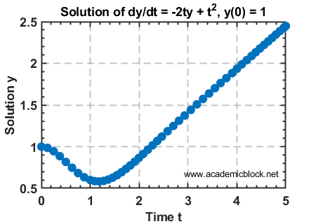
\[ \frac{dy}{dt} = -2ty + t^2, \quad y(0) = 1 \]
We aim to solve this numerically for \( t \) in the range [0, 5].
MATLAB Code
% Define the ODE function

odefun = @(t, y) -2 * t * y + t^2;


% Specify the time range and initial condition

tspan = [0 5];  % Time range from t = 0 to t = 5

y0 = 1;         % Initial condition y(0) = 1


% Solve the ODE using ode45

[t, y] = ode45(odefun, tspan, y0);


% Display the solution (time and y values)

disp([t, y]);


% Plot the solution

plot(t, y, '-o');  % Use markers for clarity

xlabel('Time t');

ylabel('Solution y');

title('Solution of dy/dt = -2ty + t^2, y(0) = 1');

grid on;
Explanation of the Code
Step 1: Define the ODE function using an anonymous function.
Step 2: Specify the time range (tspan) and initial condition (y0).
Step 3: Use MATLAB’s ode45 solver to compute the solution.
Step 4: Plot the solution for visualization.
Expected Output
When you run the code, MATLAB displays the time and solution values:
    t           y
    0.0000      1.0000
    0.1000      1.0101
    0.2000      1.0408
    0.3000      1.0912
    ...
    5.0000      52.8739
The plot will show how \( y(t) \) evolves over time for the given initial condition \( y(0) = 1 \).
Plot
The plot will depict the solution \( y(t) \) growing as \( t \) increases, influenced by the \( t^2 \) term in the equation.
Boundary Value Problems (BVPs) in MATLAB
Boundary Value Problems (BVPs) are differential equations with conditions specified at different points. MATLAB provides the bvp4c function for solving such problems numerically.
Example Problem
Consider the BVP:
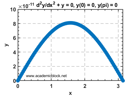
\[ \frac{d^2y}{dx^2} + y = 0, \quad y(0) = 0, \quad y(\pi) = 0 \]
We aim to solve this numerically for \( x \) in the range [0, \( \pi \)].
MATLAB Code
% Solve the BVP using bvp4c

xmesh = linspace(0, pi, 20); % Discretize the domain [0, pi]

solinit = bvpinit(xmesh, @guess); % Initialize the solution

sol = bvp4c(@bvpfun, @bcfun, solinit);


% Extract and plot the solution

x = linspace(0, pi, 100);

y = deval(sol, x);

plot(x, y(1, :), '-o'); % Plot y(x)

xlabel('x');

ylabel('y');

title('Solution of d^2y/dx^2 + y = 0, y(0) = 0, y(pi) = 0');

grid on;


% Define the BVP as a system of first-order ODEs

function dydx = bvpfun(x, y)

dydx = [y(2); -y(1)];

end


% Define the boundary conditions

function res = bcfun(ya, yb)

res = [ya(1); yb(1)]; % y(0) = 0, y(pi) = 0

end


% Initial guess for the solution

function yinit = guess(x)

yinit = [sin(x); cos(x)]; % A reasonable guess

end
Explanation of the Code
Step 1: Define the BVP as a system of first-order ODEs in bvpfun.
Step 2: Specify the boundary conditions in bcfun.
Step 3: Provide an initial guess for the solution using the guess function.
Step 4: Use bvp4c to solve the BVP.
Step 5: Extract and plot the solution for visualization.
Expected Output
Running the code will produce a plot of \( y(x) \), which oscillates within the interval [0, \( \pi \)] satisfying the boundary conditions.
Useful MATLAB Functions for ODEs
Practice Questions
Test Yourself
1. Solve dy/dt = 3y, y(0) = 1, and plot the solution.
2. Solve dy/dt = -y2 for y(0) = 1.
3. Solve the system dx/dt = x + y, dy/dt = x - y for [x(0), y(0)] = [1, -1].
4. Solve the IVP (Initial Value Problem): \[ \frac{dy}{dt} = 3y – t, \quad y(1) = 0 \] for \( t \) in the range [1, 4] using MATLAB. Visualize the result.
5. Solve the BVP: \[ \frac{d^2y}{dx^2} = -2y, \quad y(0) = 1, \quad y(1) = 0 \] for \( x \) in the range [0, 1] using MATLAB. Visualize the result.