Partial Differential Equations (PDEs) in MATLAB
Partial Differential Equations (PDEs) involve equations with partial derivatives and are widely used to describe physical phenomena such as heat transfer, fluid dynamics, and wave propagation. MATLAB offers several tools for solving PDEs, including the pdepe solver for one-dimensional problems and the PDE Toolbox for more advanced applications.
Types of PDEs
Here are some common types of PDEs:
- Parabolic PDEs: Represent diffusion processes, such as the heat equation.
- Hyperbolic PDEs: Represent wave propagation, such as the wave equation.
- Elliptic PDEs: Represent steady-state phenomena, such as Laplace’s equation.
Solving PDEs in MATLAB
Let’s explore how to solve different PDEs using MATLAB with examples.
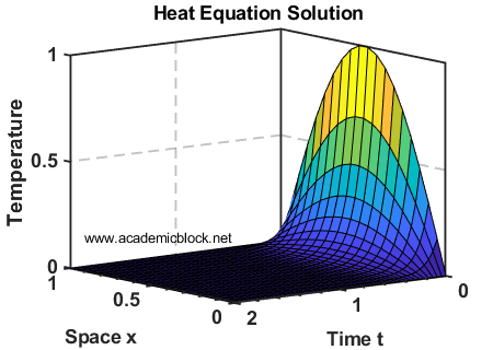
1. Heat Equation
The heat equation is a parabolic PDE given by:
∂u/∂t = α∂2u/∂x2
Here’s how to solve it using the pdepe solver:
\[ \frac{\partial u}{\partial t} = \alpha \frac{\partial^2 u}{\partial x^2} \]
% Solving the heat equation

m = 0;  % Symmetry parameter

alpha = 1;  % Diffusion coefficient


% Define PDE, initial conditions, and boundary conditions

pdefun = @(x,t,u,DuDx) alpha*DuDx;

icfun = @(x) sin(pi*x);  % Initial condition

bcfun = @(xl,ul,xr,ur,t) [ul; ur];  % Boundary condition


% Solve the PDE

x = linspace(0, 1, 20);

t = linspace(0, 2, 50);

sol = pdepe(m, pdefun, icfun, bcfun, x, t);


% Plot the solution

surf(x, t, sol);

title('Heat Equation Solution');

xlabel('Space x');

ylabel('Time t');
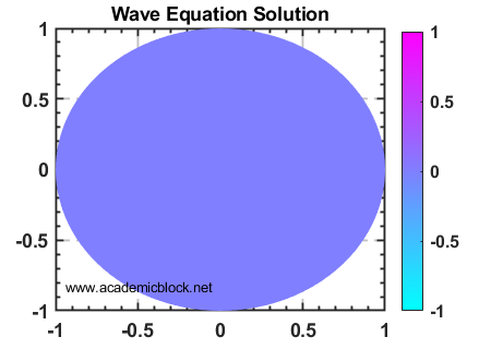
2. Wave Equation
The wave equation is a hyperbolic PDE given by:
∂2u/∂t2 = c2∂2u/∂x2
The PDE Toolbox can be used to solve this equation:
\[ \frac{\partial^2 u}{\partial t^2} = c^2 \frac{\partial^2 u}{\partial x^2} \]
% Solving the wave equation

model = createpde();


% Define geometry

geometryFromEdges(model,@circleg);


% Define PDE coefficients

specifyCoefficients(model,'m',0,'d',1,'c',1,'a',0,'f',0);


% Apply boundary and initial conditions

applyBoundaryCondition(model,'dirichlet','Edge',1:model.Geometry.NumEdges,'u',0);

setInitialConditions(model,0,0);


% Generate the mesh (fix for the error)

generateMesh(model);


% Solve the PDE

tlist = 0:0.1:2;

results = solvepde(model,tlist);


% Visualize the solution

pdeplot(model,'XYData',results.NodalSolution(:,end)); % Plot last time step

title('Wave Equation Solution');
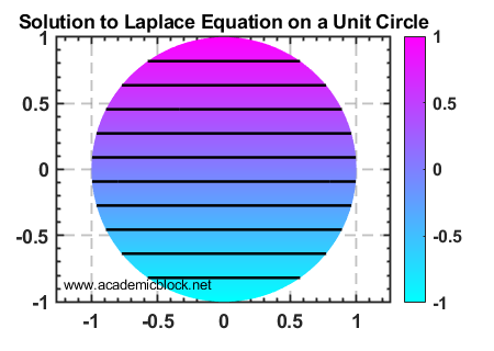
3. Laplace’s Equation
Laplace’s equation is an elliptic PDE given by:
∇2u = 0
\[ \nabla^2 u = 0 \]
% Solving Laplace’s equation

model = createpde();

geometryFromEdges(model,@circleg);  % Define geometry

specifyCoefficients(model,'m',0,'d',0,'c',1,'a',0,'f',0);  % Define coefficients


% Apply boundary conditions

applyBoundaryCondition(model,'dirichlet','Edge',1:model.Geometry.NumEdges,'u',sin(theta));


% Solve the PDE

results = solvepde(model);


% Visualize the solution

pdeplot(model,'XYData',results.NodalSolution);

title('Laplace Equation Solution');
4. Initial Value Problem (IVP): Wave Equation
Consider the wave equation with initial conditions:
∂2u/∂t2 = c2∂2u/∂x2
\[ \frac{\partial^2 u}{\partial t^2} = c^2 \frac{\partial^2 u}{\partial x^2} \]
Initial conditions:
u(x,0) = sin(πx)(initial displacement)∂u/∂t(x,0) = 0(initial velocity)
Here’s how to solve the IVP for the wave equation using MATLAB:
% Parameters

c = 1;  % Wave speed

L = 1;  % Length of the domain

x = linspace(0, L, 100);  % Space grid

t = linspace(0, 2, 200);  % Time grid


% Initial conditions

u0 = sin(pi * x);  % Initial displacement

ut0 = zeros(size(x));  % Initial velocity


% Solve the PDE using the method of lines (finite differences)

dx = x(2) - x(1);

dt = t(2) - t(1);

u = zeros(length(x), length(t));  % Initialize solution matrix

u(:,1) = u0;  % Apply initial displacement

u(:,2) = u(:,1) + dt * ut0 + 0.5 * (c * dt / dx)^2 * diff([0; u(:,1); 0], 2);


% Time-stepping loop

for n = 2:length(t)-1

    u(:,n+1) = 2 * u(:,n) - u(:,n-1) + (c * dt / dx)^2 * diff([0; u(:,n); 0], 2);

end


% Visualize the solution

[X,T] = meshgrid(x, t);

surf(X, T, u');

title('Wave Equation Solution for IVP');

xlabel('Space x');

ylabel('Time t');

zlabel('u(x,t)');
This code uses the finite difference method to solve the wave equation. The initial displacement and velocity conditions are incorporated directly into the solution.
The output is a 3D plot showing how the wave evolves over space and time.
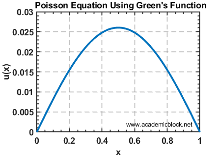
5. Solving a PDE Using Green’s Functions: Poisson’s Equation
Consider the one-dimensional Poisson equation:
-d2u/dx2 = f(x)
\[ -\frac{d^2 u}{dx^2} = f(x) \]
Boundary conditions:
u(0) = 0andu(1) = 0
The Green’s function approach involves solving the equation using:
u(x) = ∫01 G(x, ξ)f(ξ)dξ
\[ u(x) = \int_0^1 G(x, \xi) f(\xi) \, d\xi \]
where G(x, ξ) is the Green’s function satisfying the boundary conditions and the operator properties.
% Define the problem

L = 1; % Length of the domain

f = @(x) x .* (1 - x); % Source function

N = 100; % Number of points for discretization


% Discretize the domain

x = linspace(0, L, N);

dx = x(2) - x(1); % Grid spacing


% Compute the Green’s function

G = zeros(N, N);

for i = 1:N

    for j = 1:N

        if x(i) <= x(j)

            G(i, j) = x(i) * (1 - x(j));

        else

            G(i, j) = x(j) * (1 - x(i));

        end

    end

end


% Solve using Green's function

u = G * f(x)' * dx; % Integral as a matrix-vector multiplication


% Plot the results

plot(x, u, 'b-', 'LineWidth', 2);

xlabel('x');

ylabel('u(x)');

title('Solution to Poisson Equation Using Green''s Function');

grid on;
Explanation
The matrix G is constructed based on the Green’s function properties, integrating over the source function f(x). The solution u(x) is computed numerically using matrix-vector multiplication, representing the integral.
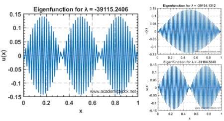
6. Solving an Eigenvalue Problem for PDEs: Vibrating String
Consider the eigenvalue problem for the vibrating string described by:
d2u/dx2 + λu = 0
\[ \frac{d^2 u}{dx^2} + \lambda u = 0 \]
Boundary conditions:
u(0) = 0andu(L) = 0
The goal is to find the eigenvalues (λ) and eigenfunctions (u(x)) for the PDE.
% Define the problem parameters

L = 1; % Length of the string

N = 100; % Number of grid points


% Discretize the domain

x = linspace(0, L, N);

dx = x(2) - x(1); % Grid spacing


% Construct the finite difference matrix (Laplacian operator)

D = diag(-2 * ones(N, 1)) + diag(ones(N - 1, 1), 1) + diag(ones(N - 1, 1), -1);

D = D / dx^2;


% Apply boundary conditions (Dirichlet: u(0) = u(L) = 0)

D(1, :) = 0;

D(N, :) = 0;

D(1, 1) = 1;

D(N, N) = 1;


% Compute eigenvalues and eigenvectors

[Eigenvectors, Eigenvalues] = eig(D);

eigenvalues = diag(Eigenvalues); % Extract eigenvalues


% Select the first few eigenfunctions and eigenvalues

num_modes = 3;

for k = 1:num_modes

    figure;

    plot(x, Eigenvectors(:, k), 'LineWidth', 2);

    title(['Eigenfunction for λ = ', num2str(eigenvalues(k))]);

    xlabel('x');

    ylabel('u(x)');

    grid on;

end
Explanation
The finite difference method is used to approximate the second derivative operator. Eigenvalues represent the natural frequencies (λ), and eigenvectors correspond to the modes of vibration (u(x)). The boundary conditions are incorporated into the discrete matrix, ensuring u(0) = u(L) = 0.
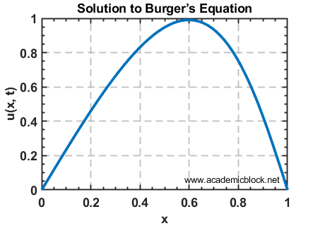
7. Solving a Nonlinear PDE: Burger’s Equation
Burger’s equation is a fundamental nonlinear PDE that combines advection and diffusion. It is expressed as:
∂u/∂t + u ∂u/∂x = ν ∂2u/∂x2
\[ \frac{\partial u}{\partial t} + u \frac{\partial u}{\partial x} = \nu \frac{\partial^2 u}{\partial x^2} \]
Where:
u(x,t): Solution variableν: Viscosity parameter
Initial condition:
u(x,0) = sin(πx)
Boundary conditions:
u(0,t) = u(1,t) = 0(Dirichlet boundary conditions)
% Define the problem parameters

L = 1; % Length of the domain

N = 100; % Number of spatial grid points

T = 0.1; % Simulation time

dt = 0.001; % Time step

nu = 0.01; % Viscosity parameter


% Discretize the spatial domain

x = linspace(0, L, N);

dx = x(2) - x(1);


% Initialize the solution

u = sin(pi * x)'; % Initial condition


% Time-stepping loop

for n = 1:round(T/dt)

    u_prev = u; % Save the previous time step

    % Update the solution using an explicit scheme

    for i = 2:N-1

        u(i) = u_prev(i) - dt * u_prev(i) * (u_prev(i+1) - u_prev(i-1)) / (2*dx) + nu * dt * (u_prev(i+1) - 2*u_prev(i) + u_prev(i-1)) / dx^2;

    end

    % Apply boundary conditions

    u(1) = 0;

    u(N) = 0;

end


% Plot the solution

figure;

plot(x, u, 'LineWidth', 2);

title('Solution to Burger’s Equation');

xlabel('x');

ylabel('u(x, t)');

grid on;
Explanation
This example uses an explicit finite difference method to solve Burger’s equation. The nonlinear term u ∂u/∂x is handled explicitly, and the diffusion term ν ∂2u/∂x2 is computed using a central difference scheme. The initial condition u(x,0) = sin(πx) evolves under the effect of advection and diffusion.
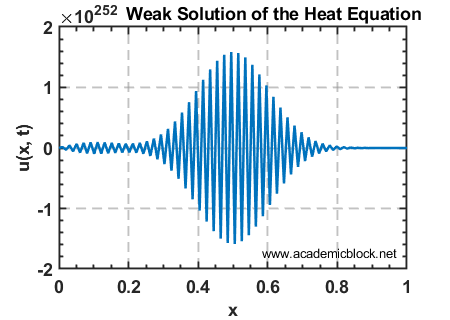
8. Weak Solutions: Solving the Heat Equation with Discontinuous Initial Data
Weak solutions are used when a PDE solution may not be differentiable in the classical sense but satisfies the equation in an integral or weak sense. Consider the heat equation:
∂u/∂t = ∂2u/∂x2
\[ \frac{\partial u}{\partial t} = \frac{\partial^2 u}{\partial x^2} \]
with the following conditions:
- Initial condition:
u(x,0) = 1for0 < x < 0.5, andu(x,0) = 0for0.5 < x < 1. - Boundary conditions:
u(0,t) = u(1,t) = 0.
We will compute the weak solution using a finite difference scheme and analyze the results.
% Define problem parameters

L = 1; % Length of the domain

N = 100; % Number of spatial points

T = 0.1; % Total simulation time

dt = 0.0005; % Time step


% Discretize the spatial domain

x = linspace(0, L, N);

dx = x(2) - x(1);


% Initialize the solution with discontinuous initial condition

u = zeros(N, 1);

u(x > 0 & x <= 0.5) = 1;


% Time-stepping loop (explicit finite difference scheme)

alpha = dt / dx^2; % Diffusion coefficient

for n = 1:round(T / dt)

    u_prev = u; % Save the previous time step

    % Update solution at interior points

    for i = 2:N-1

        u(i) = u_prev(i) + alpha * (u_prev(i+1) - 2*u_prev(i) + u_prev(i-1));

    end

    % Apply boundary conditions

    u(1) = 0;

    u(N) = 0;

end


% Plot the solution

figure;

plot(x, u, 'LineWidth', 2);

title('Weak Solution of the Heat Equation');

xlabel('x');

ylabel('u(x, t)');

grid on;
Explanation
The initial condition is discontinuous, which makes finding a classical solution challenging. Weak solutions allow the use of integral formulations or numerical methods that satisfy the PDE in an averaged sense.
The explicit finite difference scheme is used here. The term (u(i+1) - 2*u(i) + u(i-1)) models the second derivative, and the time evolution follows a simple forward Euler method. The solution smoothens over time due to diffusion, as expected for the heat equation.
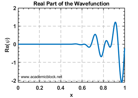
9. Quantum Mechanics: Solving the Time-Dependent Schrödinger Equation
The Schrödinger equation is a cornerstone of quantum mechanics, describing the evolution of a quantum particle. Here, we solve the one-dimensional, time-dependent Schrödinger equation:
iħ ∂ψ/∂t = -(ħ2/2m) ∂2ψ/∂x2 + V(x)ψ
\[ i\hbar \frac{\partial \psi}{\partial t} = -\frac{\hbar^2}{2m} \frac{\partial^2 \psi}{\partial x^2} + V(x)\psi \]
where:
ψ(x,t)is the wavefunction.ħis the reduced Planck’s constant.mis the particle mass.V(x)is the potential energy function.
We consider the particle in a potential well defined as:
V(x) = 0 for 0 ≤ x ≤ L, otherwise V(x) = ∞.
The initial condition is a Gaussian wave packet:
ψ(x,0) = exp(-a(x-x₀)²) * exp(i*k₀*x)
Boundary conditions are ψ(0,t) = ψ(L,t) = 0.
L = 1; % Length of the domain

N = 500; % Number of spatial points

T = 0.01; % Total simulation time

dt = 1e-5; % Time step

h = 1; % Reduced Planck's constant

m = 1; % Particle mass

a = 50; % Width of the Gaussian

xo = 0.5; % Initial position of the wave packet

ko = 50; % Wave number of the packet


% Discretize the spatial domain

x = linspace(0, L, N);

dx = x(2) - x(1);


% Initialize the wavefunction

psi = exp(-a * (x - xo).^2) .* exp(1i * ko * x);


% Potential (infinite well)

V = zeros(size(x));

V(1) = 1e10; % Large potential at boundaries to simulate an infinite well

V(end) = 1e10;


% Construct the Hamiltonian matrix (finite difference method)

H = -h^2 / (2 * m * dx^2) * (diag(ones(N-1,1),1) + diag(ones(N-1,1),-1) - 2*diag(ones(N,1))) + diag(V);


% Apply Dirichlet boundary conditions (removing first and last row/column)

H = H(2:end-1, 2:end-1);

psi = psi(2:end-1); % Remove boundary points

I = eye(N-2);


% Time evolution using Crank-Nicholson


A = I + 1i * dt / (2 * h) * H;

B = I - 1i * dt / (2 * h) * H;


for t = 0:dt:T

    psi = A \ (B * psi(:)); % Convert psi to column vector for correct multiplication

end


% Normalize the wavefunction

psi = psi / sqrt(sum(abs(psi).^2) * dx);


% Plot the real part of the wavefunction

figure;

plot(x(2:end-1), real(psi), 'LineWidth', 2); % Adjusted x-range

title('Real Part of the Wavefunction');

xlabel('x');

ylabel('Re(\psi)');

grid on;
Explanation
The time-dependent Schrödinger equation is solved numerically using the Crank-Nicholson method, which is an unconditionally stable implicit scheme. The Hamiltonian matrix H captures the kinetic energy term and the potential energy term. The wavefunction evolves in time under the operator A\B, ensuring accuracy and stability.
Useful MATLAB Functions
Practice Questions
Test Yourself
1. Solve the heat equation for different initial conditions and plot the results.
2. Solve the wave equation on a rectangular domain using the PDE Toolbox.
3. Modify Laplace’s equation to include a source term and solve it.
4. Modify the source function f(x) to sin(πx) and recompute the solution using Green’s functions.
5. Modify the boundary conditions to u'(0) = 0 (Neumann) and u(L) = 0, and compute the eigenvalues and eigenfunctions for the updated PDE.
6. For example 7, change the initial condition to u(x,0) = exp(-50*(x-0.5)^2) and analyze the evolution.